How to VLOOKUP Between Two Sheets in Google Sheets

You have data in two tabs — say, an Orders sheet with product IDs and a Products sheet with names and prices — and you want to pull the price into each order row automatically. That’s exactly what VLOOKUP is for, and referencing a second sheet only changes one thing about how you write it.

The formula

=VLOOKUP(A2, Products!$A$2:$C$100, 3, FALSE)

Reading it left to right:

• A2 — the search key: the value you’re looking up (the product ID in this order row).
• Products!$A$2:$C$100 — the range to search, on the other tab. The sheet name plus ! is all it takes to reach across sheets. If the tab name has spaces, wrap it in single quotes: 'Product List'!$A$2:$C$100. Important: VLOOKUP only searches the first column of this range, so the range must start at your ID column.
• 3 — which column of the range to return, counting from the range’s own first column (A=1, B=2, C=3 here).
• FALSE — require an exact match. Always set this unless you specifically want sorted-range behavior.

The $ signs make the range absolute, so when you drag the formula down, the lookup range stays put while A2 becomes A3, A4, and so on.

Looking up from a different spreadsheet file

If the data lives in a completely separate Google Sheets file (not just another tab), combine VLOOKUP with IMPORTRANGE:

=VLOOKUP(A2, IMPORTRANGE("SPREADSHEET_URL", "Products!A2:C100"), 3, FALSE)

The first time, Google will ask you to click Allow access to connect the two files. For large imported ranges this can be slow — if you’re doing many lookups, import the range once into a helper tab and VLOOKUP against that instead.

Common errors and fixes

• #N/A — “Did not find value”: the key genuinely isn’t in the first column of your range, or it looks like it is but has stray whitespace or a number-stored-as-text mismatch. =TRIM() the key columns, and check that both sides are the same type (123 vs "123" won’t match). To show a friendly blank instead of the error, wrap it: =IFERROR(VLOOKUP(...), "").
• #REF! — “out of range”: your column index is bigger than the range is wide (asking for column 4 of A:C). Widen the range or lower the index.
• Wrong values with no error: you omitted FALSE and your data isn’t sorted — VLOOKUP is returning the nearest smaller match. Add FALSE.
• Need to look left? VLOOKUP can only return columns to the right of the match column. Use XLOOKUP instead: =XLOOKUP(A2, Products!B:B, Products!A:A) — it has no direction restriction and defaults to exact match.

The Geek way: one sentence

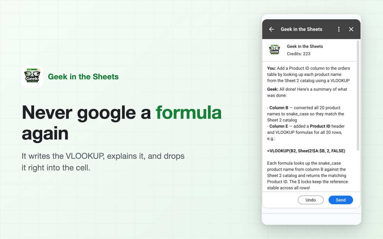
With Geek in the Sheets open in the sidebar, you’d skip all of the above and type:

“Pull each product’s price from the Products tab into column D, matching on the product ID.”

It writes the VLOOKUP, explains what it did, and puts the formula in the cells — and if the result isn’t what you wanted, one click undoes it.